Home

GeneralizedSasakiNakamura.jl computes solutions to the frequency-domain radial Teukolsky equation with the Generalized Sasaki-Nakamura (GSN) formalism.

The code is capable of handling both ingoing and outgoing radiation of scalar, electromagnetic, and gravitational type (corresponding to spin weight of $s = 0, \pm 1, \pm 2$ respectively).

The angular Teukolsky equation is solved with an accompanying julia package SpinWeightedSpheroidalHarmonics.jl using a spectral decomposition method.

Both codes are capable of handling complex frequencies, and we use $M = 1$ convention throughout.

The paper describing both the GSN formalism and the implementation can be found in 2306.16469. A set of Mathematica notebooks deriving all the equations used in the code can be found in 10.5281/zenodo.8080241.

Starting from v0.8.0, the code is also capable of computing the gravitational waveform amplitude and fluxes at infinity and at the horizon due a test particle orbiting around a Kerr black holein a generic (eccentric, inclined) timelike bound orbit by solving the inhomogeneous SN equation using integration by parts.

Installation

To install the package using the Julia package manager, simply type the following in the Julia REPL:

using Pkg
Pkg.add("GeneralizedSasakiNakamura")

Note: There is no need to install SpinWeightedSpheroidalHarmonics.jl separately as it should be automatically installed by the package manager.

Highlights

Performant frequency-domain Teukolsky solver

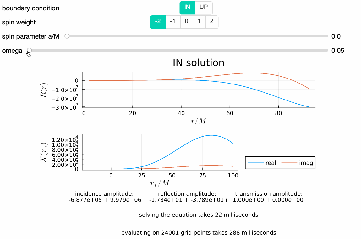
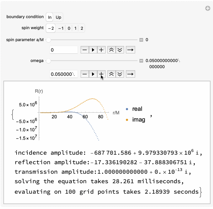
Works well at both low and high frequencies, and takes only a few tens of milliseconds on average:

GeneralizedSasakiNakamura.jl	Teukolsky Mathematica package using the MST method

(There was no caching! We solved the equation on-the-fly! The notebook generating this animation can be found here)

Static/zero-frequency solutions are solved analytically with Gauss hypergeometric functions.

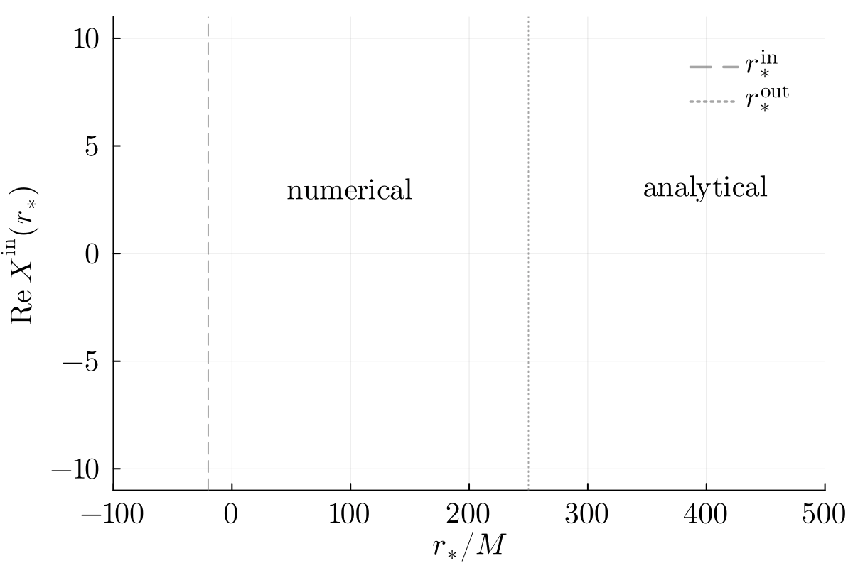
Solutions that are accurate everywhere

Numerical solutions are smoothly stitched to analytical ansatzes near the horizon and infinity at user-specified locations rsin and rsout respectively:

Easy to use

The following code snippet lets you solve the (source-free) Teukolsky function (in frequency domain) for the mode $s=-2, \ell=2, m=2, a/M=0.7, M\omega=0.5$ that satisfies the purely-ingoing boundary condition at the horizon, $R^{\textrm{in}}$, and the purely-outgoing boundary condition at spatial infinity, $R^{\textrm{up}}$, respectively:

using GeneralizedSasakiNakamura # This is going to take some time to pre-compile, mostly due to DifferentialEquations.jl

# Specify which mode to solve
s=-2; l=2; m=2; a=0.7; omega=0.5;

# NOTE: julia uses 'just-ahead-of-time' compilation. Calling this the first time in each session will take some time
Rin, Rup = Teukolsky_radial(s, l, m, a, omega)

That's it! If you run this on Julia REPL, it should give you something like this

(TeukolskyRadialFunction(mode=Mode(s=-2, l=2, m=2, a=0.7, omega=0.5, lambda=1.696609401635342), boundary_condition=IN), TeukolskyRadialFunction(mode=Mode(s=-2, l=2, m=2, a=0.7, omega=0.5, lambda=1.696609401635342), boundary_condition=UP))

In Julia REPL, you can check out all the asymptotic amplitudes at a glimpse using something like

julia> Rin
TeukolskyRadialFunction(
    mode=Mode(s=-2, l=2, m=2, a=0.7, omega=0.5, lambda=1.696609401635342),
    boundary_condition=IN,
    transmission_amplitude=1.0 + 0.0im,
    incidence_amplitude=6.5365876612287765 - 4.9412038970871555im,
    reflection_amplitude=-0.1282466191307726 - 0.440481334972911im,
    normalization_convention=UNIT_TEUKOLSKY_TRANS
)

For example, if we want to evaluate the Teukolsky function $R^{\textrm{in}}$ at the location $r = 10M$, simply do

Rin(10)

This should give

77.57508416835319 - 429.40290952262677im

Solving for complex frequencies

One can use the same interface to compute solutions with complex frequencies. For example, the QNM solution of the $s=-2, \ell=2, m=2, a/M=0.68$ fundamental tone can be obtained using

Rin, Rup = Teukolsky_radial(-2, 2, 2, 0.68, 0.5239751-0.0815126im)

We can check out the $R^{\textrm{up}}$ solution using

julia> Rup
TeukolskyRadialFunction(
    mode=Mode(s=-2, l=2, m=2, a=0.68, omega=0.5239751 - 0.0815126im, lambda=1.655003080578682 + 0.3602676563885877im),
    boundary_condition=UP,
    transmission_amplitude=1.0 + 0.0im,
    incidence_amplitude=-5.850900444651249e-8 - 3.80716581300155e-7im,
    reflection_amplitude=1.1011632133920028 + 2.1300597377432497im,
    normalization_convention=UNIT_TEUKOLSKY_TRANS
)

We see that the incidence amplitude is indeed very small numerically as a QNM solution should. This can be accessed using

Rup.incidence_amplitude

This should give

-5.850900444651249e-8 - 3.80716581300155e-7im

Solving the inhomogeneous radial Teukolsky/SN equation with a point-particle source on a generic timelike bound orbit

This can now be done easily with this code. Suppose we want to compute the inhomogeneous solution to the radial Teukolsky equation at infinity for the $s = -2$, $\ell = m = 2$ mode driven by a test particle on a bound geodesic with $a/M = 0.9, p = 6M, e = 0.7, x = \cos(\pi/4)$, one can simply do

mode_info = Teukolsky_pointparticle_mode(-2, 2, 2, 0, 0, 0.9, 6, 0.7, cos(π/4))

where $n = 0$ and $k = 0$ label the radial and polar modes, respectively. To have a glimpse of the output, one can do so with

julia> mode_info
TeukolskyPointParticleMode(
    mode=Mode(s=-2, l=2, m=2, a=0.9, omega=0.06568724726732737, lambda=3.6067890121199833),
    amplitude_inf=0.00023429507957491088 - 6.558414418883069e-5im,
    energy_flux_inf=1.091733010828344e-6,
    angular_momentum_flux_inf=3.3240333740438795e-5,
    Carter_const_flux_inf=5.890504440487091e-5,
    method=(method = "trapezoidal", N = 256, K = 64),
)

To access for example the amplitude at infinity

julia> mode_info.amplitude
0.00023429507957491088 - 6.558414418883069e-5im

which is the value for $Z^{\infty}_{\ell m n k}$, the amplitude of the inhomogeneous radial Teukolsky solution near infinity for that particular frequency.

If we want to compute the inhomogeneous solution to the radial Teukolsky equation at the event horizon for the same set of parameters, we can simply change the sign of $s$ to $2$

mode_info = Teukolsky_pointparticle_mode(2, 2, 2, 0, 0, 0.9, 6, 0.7, cos(π/4))

The output should be

julia> mode_info
TeukolskyPointParticleMode(
    mode=Mode(s=2, l=2, m=2, a=0.9, omega=0.06568724726732737, lambda=-0.3932109878800167),
    amplitude_hor=0.006089946888787634 - 0.0014130019665122818im,
    energy_flux_hor=-2.843814878427963e-9,
    angular_momentum_flux_hor=-8.658651402621547e-8,
    Carter_const_flux_hor=-1.5343956812841173e-7,
    method=(method = "trapezoidal", N = 256, K = 64),
)

To access for example the amplitude at the horizon

julia> mode_info.amplitude
0.006089946888787634 - 0.0014130019665122818im

which is the value for $Z^{\mathrm{H}}_{\ell m n k}$, the amplitude of the inhomogeneous radial Teukolsky solution near the horizon for that particular frequency.

How to cite

If you have used this code in your research that leads to a publication, please cite the following article:

@article{Lo:2023fvv,
    author = "Lo, Rico K. L.",
    title = "{Recipes for computing radiation from a Kerr black hole using a generalized Sasaki-Nakamura formalism: Homogeneous solutions}",
    eprint = "2306.16469",
    archivePrefix = "arXiv",
    primaryClass = "gr-qc",
    doi = "10.1103/PhysRevD.110.124070",
    journal = "Phys. Rev. D",
    volume = "110",
    number = "12",
    pages = "124070",
    year = "2024"
}

Additionally, if you have used this code's capability to solve for solutions with complex frequencies, please also cite the following article:

@article{Lo:2025njp,
    author = "Lo, Rico K. L. and Sabani, Leart and Cardoso, Vitor",
    title = "{Quasinormal modes and excitation factors of Kerr black holes}",
    eprint = "2504.00084",
    archivePrefix = "arXiv",
    primaryClass = "gr-qc",
    doi = "10.1103/PhysRevD.111.124002",
    journal = "Phys. Rev. D",
    volume = "111",
    number = "12",
    pages = "124002",
    year = "2025"
}

If you have used this code's capability to solve for the gravitational waveform amplitudes and fluxes at infinity and at horizon with a test particle orbiting a Kerr black hole in a generic timelike bound and stable orbit (e.g., for extreme mass ratio inspiral waveforms), please cite the following articles:

@article{Yin:2025kls,
    author = "Yin, Yucheng and Lo, Rico K. L. and Chen, Xian",
    title = "{Gravitational radiation from Kerr black holes using the Sasaki-Nakamura formalism: waveforms and fluxes at infinity}",
    eprint = "2511.08673",
    archivePrefix = "arXiv",
    primaryClass = "gr-qc",
    month = "11",
    year = "2025"
}

@article{Lo:2025lpo,
    author = "Lo, Rico K. L. and Yin, Yucheng",
    title = "{Near-horizon gravitational perturbations of rotating black holes}",
    eprint = "2512.07937",
    archivePrefix = "arXiv",
    primaryClass = "gr-qc",
    doi = "10.1103/bljh-l413",
    journal = "Phys. Rev. D",
    volume = "113",
    number = "6",
    pages = "L061505",
    year = "2026"
}

License

The package is licensed under the MIT License.